Probabilistic Sensitivity Analysis
Fernando Alarid-Escudero, Greg Knowlton, Eva Enns, and the DARTH Team
2026-11-17
Source:vignettes/psa_analysis.Rmd
psa_analysis.RmdOverview
The probabilistic sensitivity analysis (PSA) object is a key part of
the dampack package. In this vignette, we discuss the goals
of a probabilistic sensitivity analysis, how to create the
dampack PSA object from an existing PSA dataset, and what
can be done once the PSA object is created in dampack.
dampack has additional functionality for generating a
PSA dataset with a user-defined R-based decision model and specified
parameter distributions. Those methods are covered in the
psa_generation vignette (type
vignette("psa_generation", package = "dampack") in the
console after installing the dampack package). Even if you
intend to generate your own PSA dataset using dampack, it
is recommended that you continue reading this vignette
(psa_analysis) first.
Probability Sensitivity Analysis: An Introduction
The purpose of a PSA is to translate model parameter uncertainty into decision uncertainty, measured as the probability that a given strategy is optimal. In the context of cost-effectiveness analysis, this is the probability that a given strategy is cost-effective, defined as achieving the maximum health benefit at a cost per unit benefit gained less than a defined maximum willingness-to-pay (WTP) per unit benefit. The cost-effective strategy is equivalently defined as the strategy that maximizes the net monetary benefit (NMB) calculated as WTP * Benefit - Cost, with an appropriately set WTP. Thus, in the PSA examples, we will generally use NMB as the outcome of each strategy.
Parameter uncertainty is reflected in probability distributions defined for each model parameter. Common distributions include the normal, beta, gamma, and log-normal distributions. To generate a single PSA sample, a value is randomly drawn for each parameter from its respective distribution. The model is then run for that set of parameter values to calculate the resulting outcomes of interest for each strategy. A large number of PSA samples, say 10,000, are generated in this way, with each iteration using one set of values from the distributions of the parameters and each iteration yielding one set of outcome values. The resulting distribution of outcome values across the PSA samples translates into decision uncertainty when certain strategies are favored in some samples but not in others.
For a more in-depth discussion of cost-effectiveness analysis and the role of PSA, we recommend the following readings: - Alarid-Escudero, Fernando, Eva A. Enns, Karen M. Kuntz, Tzeyu L. Michaud, and Hawre Jalal. “Time traveling is just too dangerous” but some methods are worth revisiting: the advantages of expected loss curves over cost-effectiveness acceptability curves and frontier. Value in Health 2019; 22(5):611-618. - Cost-Effectiveness in Health and Medicine, 2nd edition, eds: Neumann PJ, Ganiats TG, Russell LB, Sanders GD, Siegel JE. Oxford University Press, 2016.
Creating the psa object
The psa object is created using the function
make_psa_obj, which requires at minimum cost
and effectiveness arguments. These two arguments must be
data.frames of the same dimension, with columns
corresponding to strategies and rows corresponding to PSA samples. The
strategies argument expects a character vector of strategy
names (listed in the same order as the data.frame columns). If
strategeies names are not explicitly provided, they will be labeled in
sequential order (i.e. Strategy_1, Strategy_2, etc.). These inputs are
sufficient for basic PSA-based functions within
dampack.
However, for more advanced functionality for deriving one- and
two-way sensitivity analyses from the PSA, the parameters
argument should be provided with a data.frame containing
the value of each parameter (columns) used in each PSA sample (rows).
The column names should be the parameter names.
As additional options, the user can provide an alternate currency
symbol (to the “$” default) for labeling using the currency
argument. A data.frame of a third outcome of interest (of
the same structure as costs and effectiveness data.frames)
can also optionally be provided to the other_outcome
argument.
Read in data
Within dampack there is an example PSA dataset from a
model evaluating different cancer treatments. We will use this dataset
to illustrate the construction of a psa object to which we
will apply the analysis and visualization functions included in
dampack.
We can see the structure of the data with str():
str(cancer_psa_data)
#> List of 4
#>  $ strategies   : chr [1:3] "Chemo" "Radio" "Surgery"
#>  $ cost         :'data.frame':   10000 obs. of  3 variables:
#>   ..$ Chemo_Cost: num [1:10000] 33683 30131 26839 28671 31540 ...
#>   ..$ Radio_Cost: num [1:10000] 8942 19705 13250 21505 13163 ...
#>   ..$ Surg_Cost : num [1:10000] 29706 28565 22430 28498 12835 ...
#>  $ effectiveness:'data.frame':   10000 obs. of  3 variables:
#>   ..$ Chemo_Eff: num [1:10000] 12.73 9.85 10.05 11.68 10.76 ...
#>   ..$ Radio_Eff: num [1:10000] 12.13 9.86 10.01 11.01 10.75 ...
#>   ..$ Surg_Eff : num [1:10000] 11.26 10.19 9.83 10.86 10.57 ...
#>  $ parameters   :'data.frame':   10000 obs. of  8 variables:
#>   ..$ pFailChemo : num [1:10000] 0.391 0.425 0.458 0.474 0.484 ...
#>   ..$ pFailRadio : num [1:10000] 0.501 0.418 0.455 0.557 0.47 ...
#>   ..$ pFailSurg  : num [1:10000] 0.1264 0.036 0.0433 0.0487 0.0531 ...
#>   ..$ pDieSurg   : num [1:10000] 0.0989 0.0876 0.1389 0.1426 0.1178 ...
#>   ..$ muDieCancer: num [1:10000] 0.113 0.285 0.257 0.15 0.201 ...
#>   ..$ cChemo     : num [1:10000] 22569 21018 17874 17687 19810 ...
#>   ..$ cRadio     : num [1:10000] 5307 13925 8927 12215 8492 ...
#>   ..$ cSurg      : num [1:10000] 29706 28565 22430 28498 12835 ...
We see that the cancer_psa_data dataset is a list that
contains:
-
strategies: a vector of strategy names. In this example, we see that there are three strategies, corresponding to three different cancer treatments.
cancer_psa_data$strategies
#> [1] "Chemo" "Radio" "Surgery"-
cost: a data frame of the cost of each strategy for each PSA sample. We see that there are three columns, one for each strategy. There are no requirements on the column names of this data frame, but it is critical these columns be in the same order as thestrategiesvector. There are 10,000 rows (the number of PSA samples).
head(cancer_psa_data$cost)
#>   Chemo_Cost Radio_Cost Surg_Cost
#> 1   33682.76   8942.488  29705.66
#> 2   30130.87  19704.842  28565.46
#> 3   26838.94  13249.548  22429.61
#> 4   28671.30  21505.019  28498.20
#> 5   31540.26  13163.105  12835.14
#> 6 32618.48 17059.544 42954.16-
effectiveness: a data frame of the effectiveness outcome (such as quality-adjusted life-years). This data frame has the same structure as thecostsdata frame, with three columns (one for each strategy) and 10,000 rows (the number of PSA samples)
head(cancer_psa_data$effectiveness)
#>   Chemo_Eff Radio_Eff  Surg_Eff
#> 1  12.72801 12.130626 11.263131
#> 2   9.85347  9.855394 10.193810
#> 3  10.05273 10.011711  9.831964
#> 4  11.67804 11.013624 10.856675
#> 5  10.75947 10.753719 10.574672
#> 6 12.30980 11.816024 11.984267-
parameters: a data frame of the parameter values used in each PSA sample. Each column represents an input parameter varied in the PSA and is named after that parameter. There are 8 columns, meaning that in this PSA, 8 parameters were varied probabilistically. The data frame has 10,000 rows, again reflecting the number of PSA samples.
head(cancer_psa_data$parameters)
#>   pFailChemo pFailRadio  pFailSurg   pDieSurg muDieCancer   cChemo    cRadio
#> 1  0.3910446  0.5007895 0.12638307 0.09893673   0.1128471 22569.12  5307.441
#> 2  0.4249714  0.4176121 0.03603596 0.08764193   0.2853686 21018.23 13924.656
#> 3  0.4575689  0.4546113 0.04333928 0.13890528   0.2573386 17874.37  8926.632
#> 4  0.4742443  0.5573990 0.04865145 0.14257438   0.1504732 17687.32 12215.145
#> 5  0.4835018  0.4704875 0.05307872 0.11784562   0.2009021 19810.28  8491.707
#> 6  0.4033608  0.4863672 0.09268298 0.04083940   0.1334748 21747.02 10426.239
#>      cSurg
#> 1 29705.66
#> 2 28565.46
#> 3 22429.61
#> 4 28498.20
#> 5 12835.14
#> 6 42954.16
Construct PSA object
We will now construct a psa object from this example
data. We do so using the make_psa_obj function.
psa_cancer <- make_psa_obj(cost = cancer_psa_data$cost,
                        effectiveness = cancer_psa_data$effectiveness,
                        parameters = cancer_psa_data$parameters,
                        strategies = cancer_psa_data$strategies,
                        currency = "$")
str(psa_cancer)
#> List of 9
#>  $ n_strategies : int 3
#>  $ strategies   : chr [1:3] "Chemo" "Radio" "Surgery"
#>  $ n_sim        : int 10000
#>  $ cost         :'data.frame':   10000 obs. of  3 variables:
#>   ..$ Chemo  : num [1:10000] 33683 30131 26839 28671 31540 ...
#>   ..$ Radio  : num [1:10000] 8942 19705 13250 21505 13163 ...
#>   ..$ Surgery: num [1:10000] 29706 28565 22430 28498 12835 ...
#>  $ effectiveness:'data.frame':   10000 obs. of  3 variables:
#>   ..$ Chemo  : num [1:10000] 12.73 9.85 10.05 11.68 10.76 ...
#>   ..$ Radio  : num [1:10000] 12.13 9.86 10.01 11.01 10.75 ...
#>   ..$ Surgery: num [1:10000] 11.26 10.19 9.83 10.86 10.57 ...
#>  $ other_outcome: NULL
#>  $ parameters   :'data.frame':   10000 obs. of  8 variables:
#>   ..$ pFailChemo : num [1:10000] 0.391 0.425 0.458 0.474 0.484 ...
#>   ..$ pFailRadio : num [1:10000] 0.501 0.418 0.455 0.557 0.47 ...
#>   ..$ pFailSurg  : num [1:10000] 0.1264 0.036 0.0433 0.0487 0.0531 ...
#>   ..$ pDieSurg   : num [1:10000] 0.0989 0.0876 0.1389 0.1426 0.1178 ...
#>   ..$ muDieCancer: num [1:10000] 0.113 0.285 0.257 0.15 0.201 ...
#>   ..$ cChemo     : num [1:10000] 22569 21018 17874 17687 19810 ...
#>   ..$ cRadio     : num [1:10000] 5307 13925 8927 12215 8492 ...
#>   ..$ cSurg      : num [1:10000] 29706 28565 22430 28498 12835 ...
#>  $ parnames     : chr [1:8] "pFailChemo" "pFailRadio" "pFailSurg" "pDieSurg" ...
#>  $ currency     : chr "$"
#>  - attr(*, "class")= chr [1:2] "psa" "sa"
psa_cancer is a psa object, which is
structured as a list with its own specialized functionality for
visualization and analysis.
A user can plot a psa object, which generates a ggplot
showing the cost vs. effectiveness scatter plot of PSA samples,
color-coded by strategy. Input options for plotting psa
objects can be displayed by typing ?plot.psa in the
console. Each point in the plot represents the the cost and
effectiveness of a specific strategy for a single sample of the PSA. The
ellipses (shown by default) helps to visualize the clustering of PSA
samples under each strategy on the cost-effectiveness plane.
plot(psa_cancer)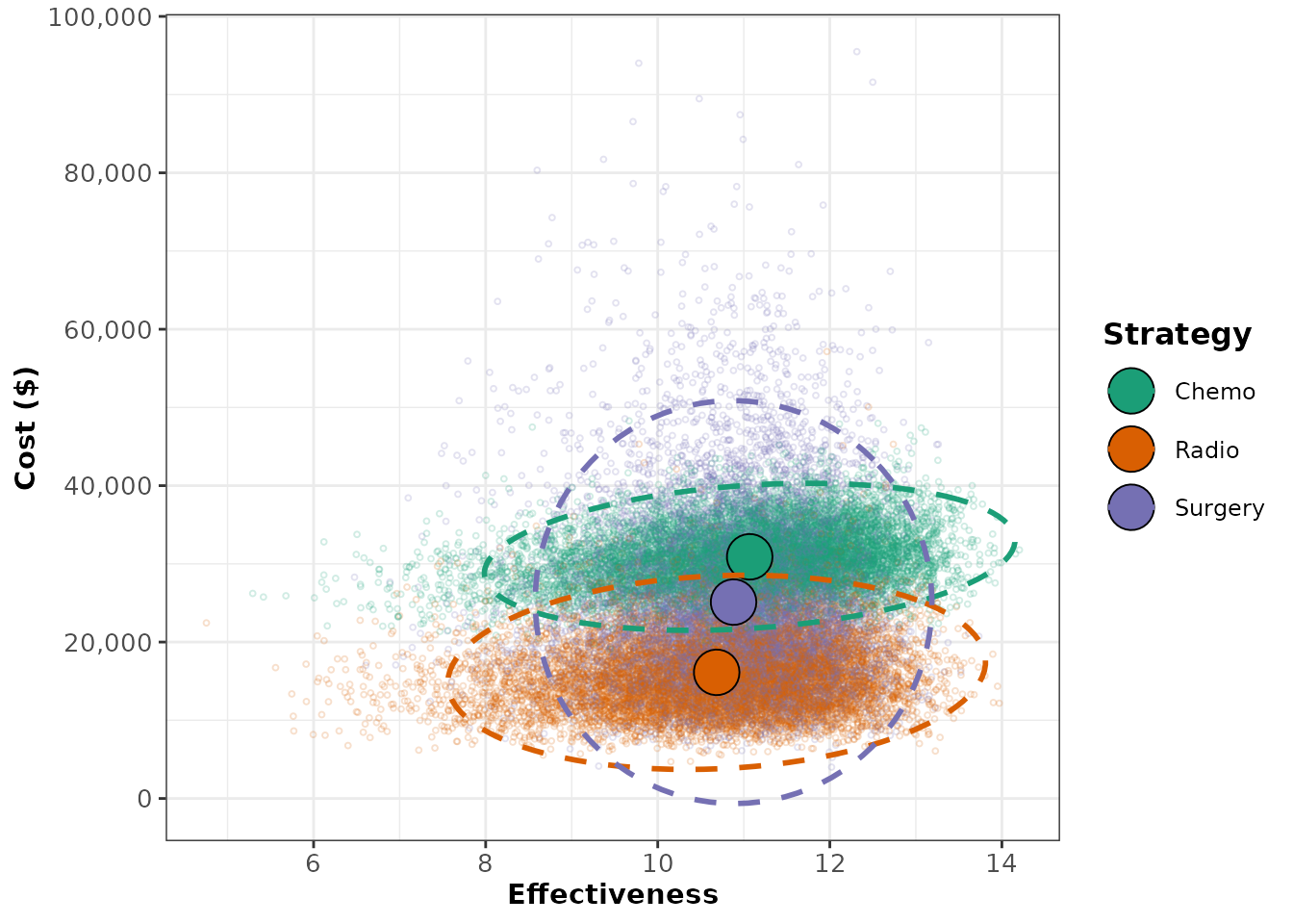
One can also visualize a scatter plot of cost and effectiveness
outcomes for each strategy incremental to a reference strategy by
passing the name of the reference strategy to the ref_str
argument. The strategy name must exactly match the spelling and case of
the strategy names within the psa object. Below, we use the
chemotherapy strategy (named “Chemo” within the psa object)
as the reference. Presenting the outcomes for the remaining strategies
in reference to the chemotherapy strategy, we can clearly see that
cost-effectiveness outcomes for the radiation and surgery treatments
generally fall in the southwest quadrant, meaning that these strategies
tend to cost less but also achieve lower health benefits than the
chemotherapy strategy.
plot(psa_cancer, ref_str = "Chemo") # Selects the "Chemo" strategy as reference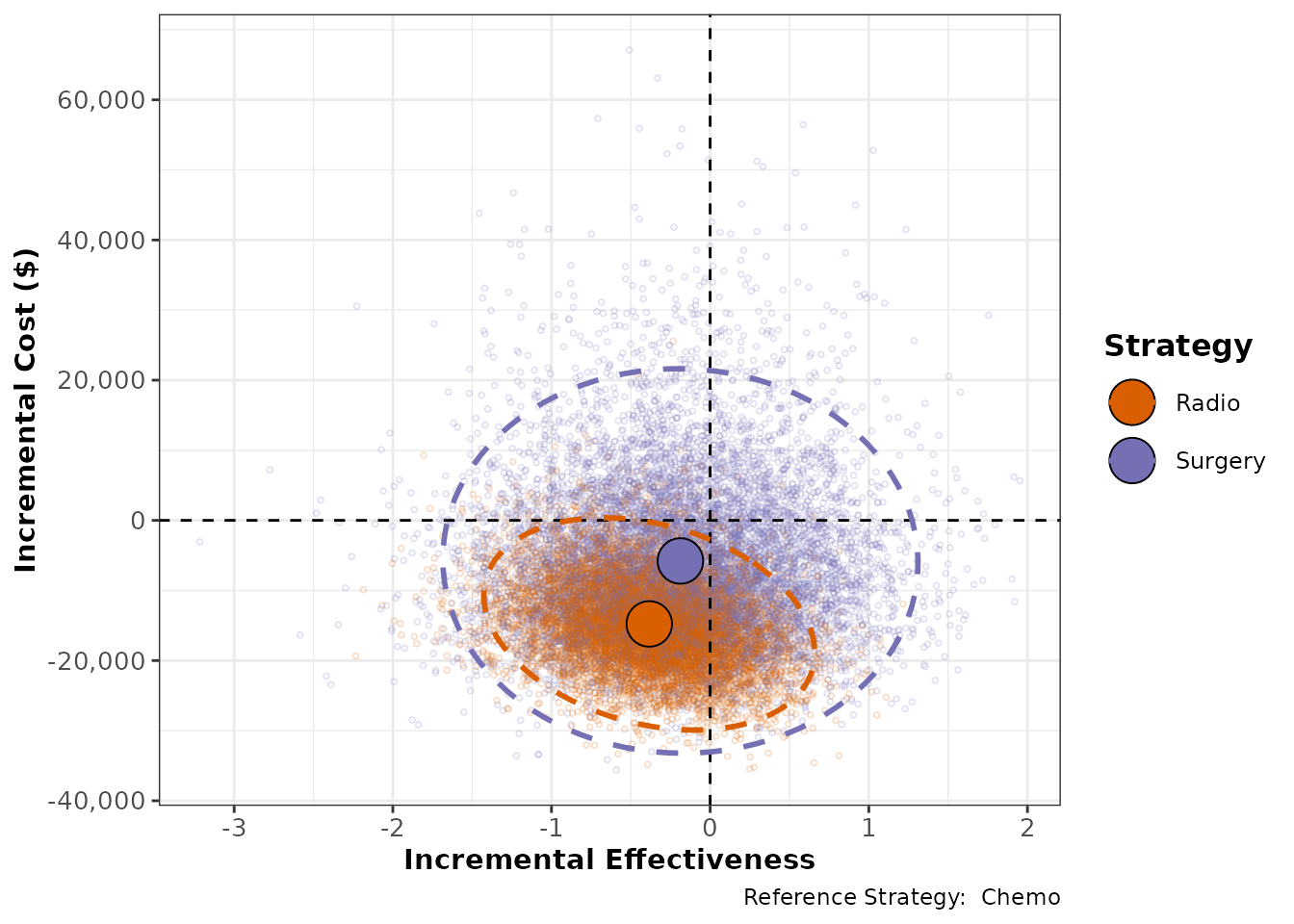
When you call summary() on a psa object, a
data.frame is returned that displays the mean cost and mean effect
across all of the PSA samples for each strategy. If
calc_sds is set to TRUE, then the standard
deviations for these outcomes are displayed as well.
psa_sum <- summary(psa_cancer,
                   calc_sds = TRUE)
psa_sum
#>   Strategy meanCost meanEffect    sdCost  sdEffect
#> 1    Chemo 30900.80   11.06869  3841.172 1.2599541
#> 2    Radio 16128.88   10.68492  5073.654 1.2768415
#> 3  Surgery 25110.22   10.88120 10523.753 0.9418639
Mean cost and effectiveness outcomes from a PSA can be analyzed
incrementally using the calculate_icers function. For a
more detailed explanation of incremental cost-effectiveness analysis,
please see the basic_cea vignette.
icers_cancer <- calculate_icers(cost = psa_sum$meanCost,
                         effect = psa_sum$meanEffect,
                         strategies = psa_sum$Strategy)
plot(icers_cancer)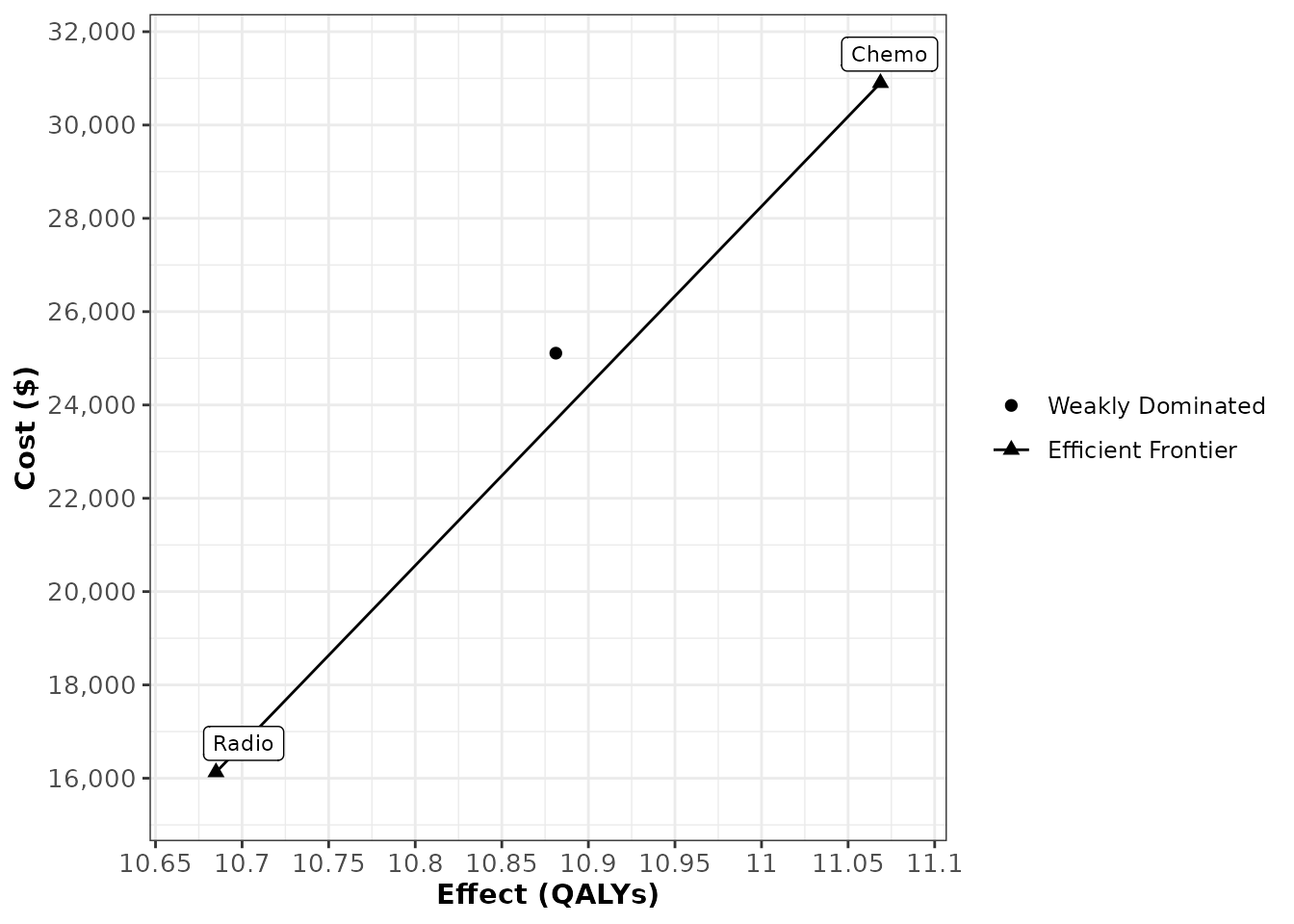
Cost-effectiveness Acceptability Curve
Results of a PSA are often displayed as a cost-effectiveness acceptability curve (CEAC), which plots the probability that each strategy is cost-effective as a function of willingness-to-pay (WTP). The CEAC translates the parameter uncertainty into decision uncertainty, showing how confident a decision maker might be that at a given strategy is cost-effective. The probability of being cost-effective is calculated as the proportion of PSA samples for which a given strategy achieves the greatest health benefit at a cost per unit of health gained less than the WTP or, equivalently, the strategy that maximizes net monetary benefit at that WTP.
The ceac() function takes as inputs a psa
object and a numeric vector of willingness to pay thresholds to create a
ceac object, which is structured as a data frame with its
own specialized functionality for visualization and analysis. The
proportion column of the ceac object is the proportion of
PSA samples in which that particular strategy had the maximum benefit at
the corresponding WTP. The On_Frontier column indicates
whether a strategy was on the cost-effectiveness acceptability frontier
at the corresponding WTP. A strategy is on the cost-effectiveness
acceptability frontier if it maximizes expected benefit on
average across all samples of the PSA at the WTP being considered.
Note that this designation is fundamentally different than identifying
the strategy that has the highest probability of being cost-effective
across all samples of the PSA. Using the summary() function
on a ceac object yields a data.frame that reports the
strategies that are on the cost-effectiveness acceptability frontier
along with the ranges of WTP values for which these optimal strategies
are most cost-effective.
WTP is the maximum amount a decision-maker is willing to pay for a one unit of health benefit gained (usually a QALY).
A strategy’s cost-effectiveness is sometimes discussed in terms of either net health benefit or net monetary benefit. To calculate a strategy’s net health benefit, the cost associated with the strategy is divided by the willingness-to-pay threshold (WTP) and added to the QALYs gained, and to calculate a strategy’s net monetary benefit, the number of QALYs gained is multiplied by the WTP threshold and added to the cost. Describing strategies in terms of net health benefit or net monetary benefit is convenient because it allows one to compare the cost-effectiveness of the strategies using a single metric, but these comparisons are sometimes very sensitive to the exact WTP threshold that is used to convert QALYs to currency, or vice versa. The degree to which the choice of willingness-to-pay threshold influences the decision can be analyzed using a cost-effectiveness acceptability curve. The acceptability curves plot the relative frequency or probability that each strategy is cost-effective compared to the alternatives for varying values for society’s willingness-to-pay.
ceac_cancer <- ceac(wtp = seq(0,250000,by=50000),
                 psa = psa_cancer)
head(ceac_cancer)
#>     WTP Strategy Proportion On_Frontier
#> 1     0    Chemo     0.0064       FALSE
#> 2     0    Radio     0.7880        TRUE
#> 3     0  Surgery     0.2056       FALSE
#> 4 50000    Chemo     0.3561        TRUE
#> 5 50000    Radio     0.2752       FALSE
#> 6 50000  Surgery     0.3687       FALSE

summary(ceac_cancer)
#>   range_min range_max optimal_strategy
#> 1         0     50000            Radio
#> 2     50000    250000            Chemo
Plotting a ceac object creates the standard
cost-effectiveness acceptability curve plot, showing the probability
that each strategy is cost-effective (y-axis) as a function of WTP
(x-axis). By default, the cost-effectiveness acceptability curve
frontier is shown. For all plotting options, see
?plot.ceac.
plot(ceac_cancer)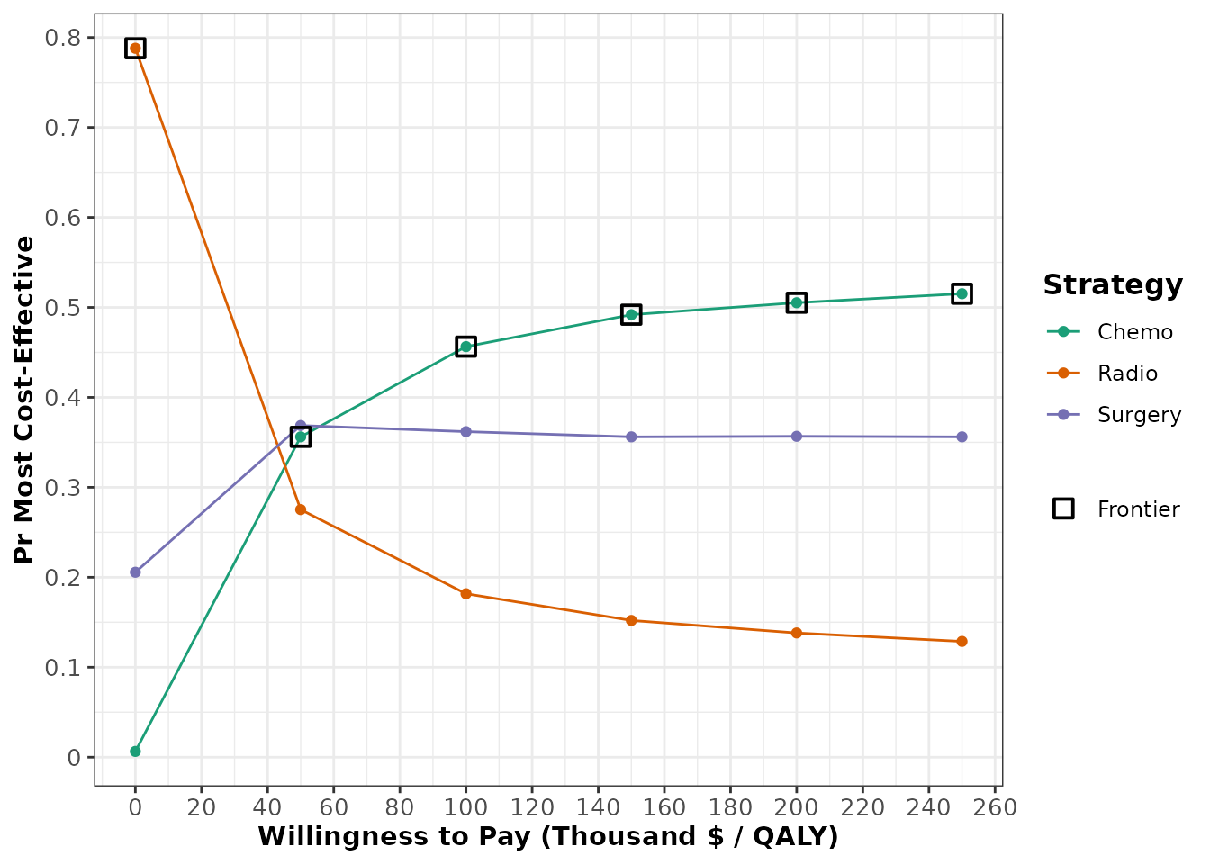
Expected Loss Curve
Alternatively, the degree to which cost-effectiveness varies with respect to the WTP threshold can be visualized using an expected loss curve (ELC). Expected loss is a quantification of the consequences of choosing a suboptimal strategy in terms of expected foregone benefits. The strategy that minimizes the expected loss at a given WTP value is the optimal decision given current information, and consequently the graph’s relationship to the cost-effectiveness acceptability frontier is somewhat more intutive than for CEACs. For an in-depth discussion on the advantages of ELCs in cost-effectiveness analysis, please refer to:
Alarid-Escudero F, Enns EA, Kuntz KM, Michaud TL, Jalal H. “Time Traveling Is Just Too Dangerous” But Some Methods Are Worth Revisiting: The Advantages of Expected Loss Curves Over Cost-Effectiveness Acceptability Curves and Frontier. Value Health. 2019;22(5):611-618.
elc_cancer <- calc_exp_loss(wtp = seq(0,250000,by=50000),
                    psa = psa_cancer)
head(elc_cancer)
#>     WTP Strategy Expected_Loss On_Frontier
#> 1     0    Chemo     15804.739       FALSE
#> 2     0    Radio      1032.819        TRUE
#> 3     0  Surgery     10014.157       FALSE
#> 4 50000    Chemo     14954.055        TRUE
#> 5 50000    Radio     19370.478       FALSE
#> 6 50000  Surgery     18537.637       FALSE
plot(elc_cancer,
     n_x_ticks = 8,
     n_y_ticks = 6)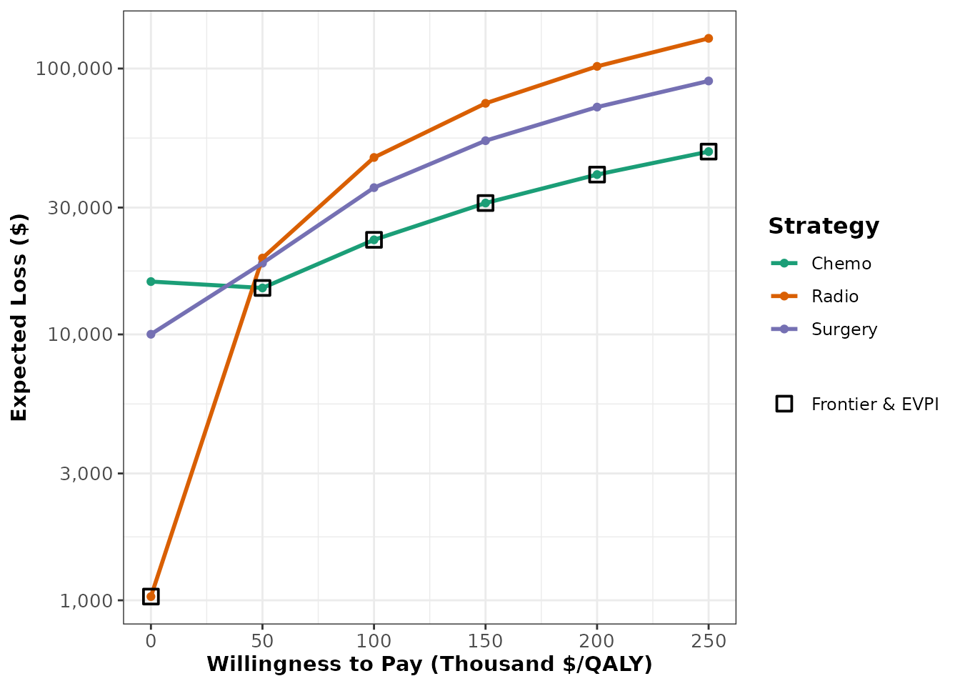
One-way Sensitivity Analysis
A one-way sensitivity analysis (OWSA) illustrates how the expected
outcome of a decision model changes as function of a single input
parameter in the PSA. Knowing that the parameters in a decision model
can interact in complex and nonlinear ways to influence outcomes, the
characterization of the role of a single parameter is not
straightforward. To disentangle the effect of the parameter of interest,
a regression model, or ‘metamodel’, is fit using the entire PSA that
treats the specified outcome (Net-monetary benefit, QALYs, etc) as the
dependent variable and the parameter as the independent variable. By
omitting the other input parameters in the PSA in the regression model,
the variation in the outcome that cannot be directly attributed to
variation in the parameter of interest is treated as random statistical
error (even if the model is purely deterministic). Consequently, any
predicted outcome value derived from the metamodel is essentially
conditional on the average value of all the other PSA parameters.
Separate models are produced for each strategy included in the
strategies argument of the owsa() function,
and these models are used to predict outcome values over a range values
of the parameter of interest.
The first input of the owsa() function is
sa_obj, which stands for “sensitivity analysis object”,
because the owsa() function can also be used in the context of a
determinstic sensitivity analysis on a dsa object. For an
illustration of this functionality, enter
vignette("dsa_generation", package = "dampack") in the
console. The params argument allows the user to execute a
series of separate one-way sensitivity analyses with a single function
call by specifying a vector of different parameters of interest. By
default, the regression model used to quantify the effect of the
parameter of interest on the expected outcome value is a second order
polynomial linear model. The order of the polynomial in the regression
model can be altered by changing the argument poly.order. A
higher value of poly.order will yield a more flexible
metamodel, which can potentially lead to overfitting.
oneway_sa_cancer <- owsa(psa_cancer)The output of the owsa() function has customized
plotting functionality that can be explored by typing
?plot.owsa in the console. Like all other plots produced by
dampack, plots derived from the owsa object
are ggplot objects and can be readily customized.
plot(oneway_sa_cancer,
     n_x_ticks = 2)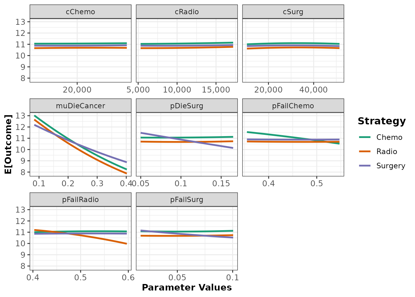
Tornado Plot
Using the owsa() function on a PSA object will produce
an owsa class object, and this object is compatible with
two special plotting functions in addition to plot.owsa().
The first of these plotting functions is owsa_tornado,
which produces a tornado plot. A tornado plot is a visual aid used to
identify which parameters are driving most of the variation in a
specified model outcome. In addition, the plot shows whether high or low
expected outcome values result from parameter values that are above or
below the median value of the parameter in question (indicated by the
fill color corresponding to “Parameter Level High/Low”. For example, the
tornado plot below tells us that the parameter
"muDieCancer" has the most leverage in affecting the
effectiveness model outcome, and that values below the median value of
"muDieCancer" in the one-way sensitivity analysis are
associated with higher expected effectiveness outcomes.
It is important to note that some important information is obscured by tornado plots and caution should be exercised when interpreting it. As the parameter of interest varies across its range in the one-way sensitivity, the strategy that maximizes the outcome of interest can also change across this range. The plot is not showing how the expected outcome changes for a single strategy, but how the expected outcome of the optimal strategy changes. The designation of which strategy is optimal is liable to alternate over the range of the parameter of interest, and this is hidden in a tornado plot.
owsa_tornado(oneway_sa_cancer)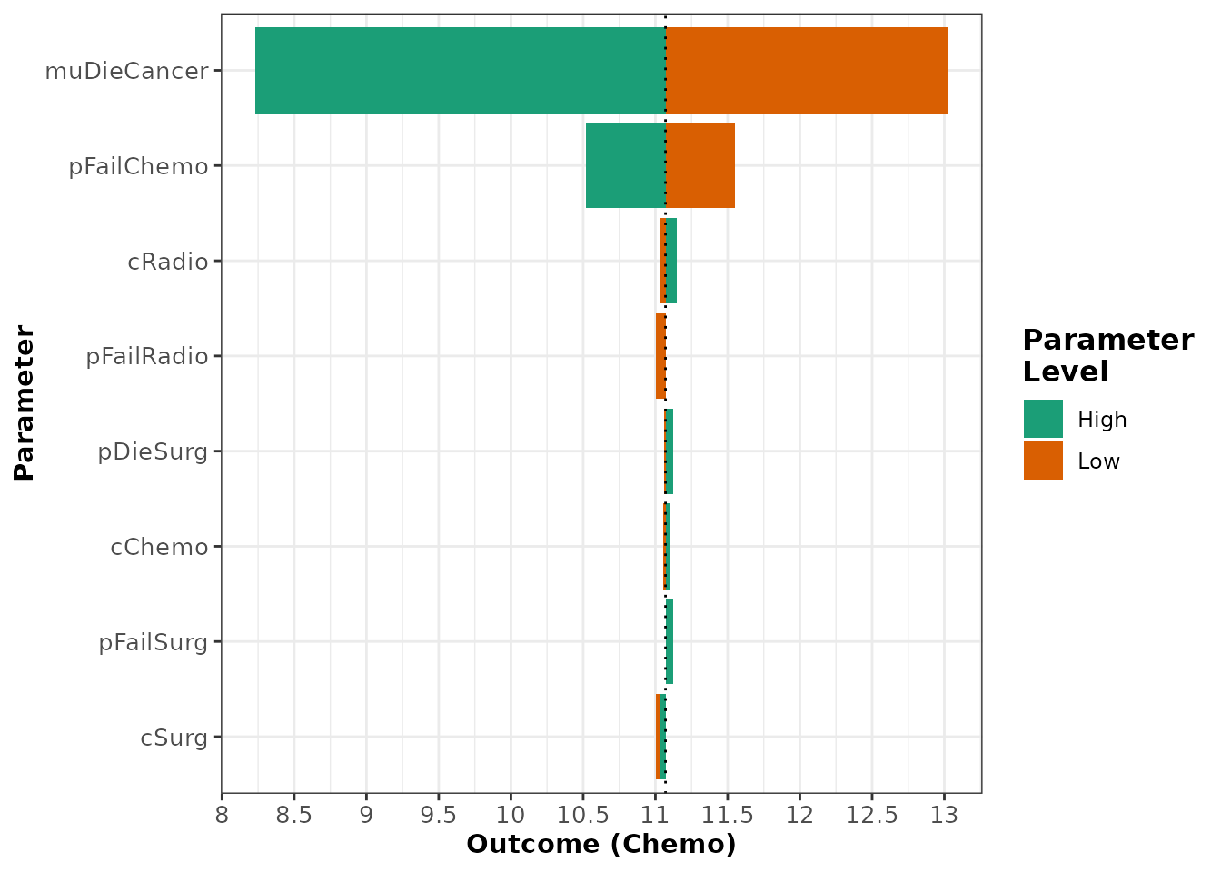
For owsa objects that contain many parameters that have minimal
effect on the parameter of interest, you may want to consider producing
a plot that highlights only the most influential parameters. Using the
min_rel_diff argument, you can instruct
owsa_tornado to exclude all parameters that fail to produce
a relative change in the outcome below a specific fraction.
owsa_tornado(oneway_sa_cancer,
min_rel_diff = 0.05)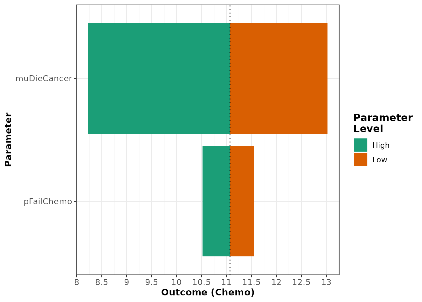 In order to attain the data.frame used to produce the tornado plot, use
the
return argument to change the type of object returned
by the owsa_tornado function.
owsa_tornado(oneway_sa_cancer,
             return = "data")
#> # A tibble: 8 × 7
#> # Groups:   parameter [8]
#>   parameter   param_val.low outcome_val.low param_val.high outcome_val.high
#>   <chr>               <dbl>           <dbl>          <dbl>            <dbl>
#> 1 muDieCancer        0.0837            13.0          0.402             8.23
#> 2 pFailChemo         0.355             11.6          0.547            10.5
#> 3 cRadio          5315.                11.0      17203.               11.1
#> 4 pFailRadio         0.403             11.0          0.597            11.1
#> 5 pDieSurg           0.0498            11.1          0.165            11.1
#> 6 cChemo         16291.                11.1      24289.               11.1
#> 7 pFailSurg          0.0168            11.1          0.100            11.1
#> 8 cSurg          10474.                11.0      51427.               11.0
#> # ℹ 2 more variables: abs_diff <dbl>, rel_diff <dbl>
Optimal Strategy Plot
The second special plotting function designed for the visualization
of the owsa object is owsa_opt_strat, which
directly addresses the crucial information that is missing from the
tornado plot. The output of owsa_opt_strat allows us to see
how the strategy that maximizes the expectation of the outcome of
interest changes as a function of each parameter of interest.
owsa_opt_strat(oneway_sa_cancer,
               n_x_ticks = 5)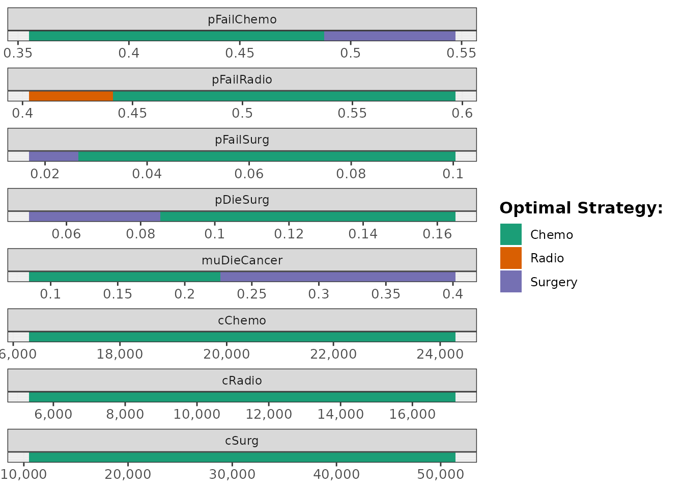
Like owsa_tornado(), the return argument in
owsa_opt_strat() allows the user to access a tidy
data.frame that contains the exact values used to produce the plot.
owsa_opt_strat(oneway_sa_cancer,
               return = "data")
#> # A tibble: 13 × 4
#>    parameter   strategy       pmin       pmax
#>    <fct>       <fct>         <dbl>      <dbl>
#>  1 cChemo      Chemo    16291.     24289.
#>  2 cRadio      Chemo     5315.     17203.
#>  3 cSurg       Chemo    10474.     51427.
#>  4 muDieCancer Chemo        0.0837     0.225
#>  5 muDieCancer Surgery      0.228      0.402
#>  6 pDieSurg    Chemo        0.0859     0.165
#>  7 pDieSurg    Surgery      0.0498     0.0847
#>  8 pFailChemo  Chemo        0.355      0.487
#>  9 pFailChemo  Surgery      0.489      0.547
#> 10 pFailRadio  Chemo        0.442      0.597
#> 11 pFailRadio  Radio        0.403      0.440
#> 12 pFailSurg   Chemo        0.0269     0.100
#> 13 pFailSurg   Surgery      0.0168     0.0261
Two-way Sensitivty Analysis
A two-way sensitivity analysis (TWSA) illustrates how the expected
outcome of a decision-analytic model changes as function of two input
parameters in the PSA. Just as a regression metamodel was used to
isolate the effect of a single parameter in dampack’s
owsa function, twsa() uses a polynomial
regression metamodel that includes both of the specified parameters to
predict the expected outcome as a function of the two parameters. This
regression metamodel includes polynomial terms up to and including the
degree of the poly.order argument for both parameters, as
well as all interaction terms between these polynomial terms.
twoway_sa_cancer <- twsa(psa_cancer,
                         param1 = "pFailChemo",
                         param2 = "muDieCancer")
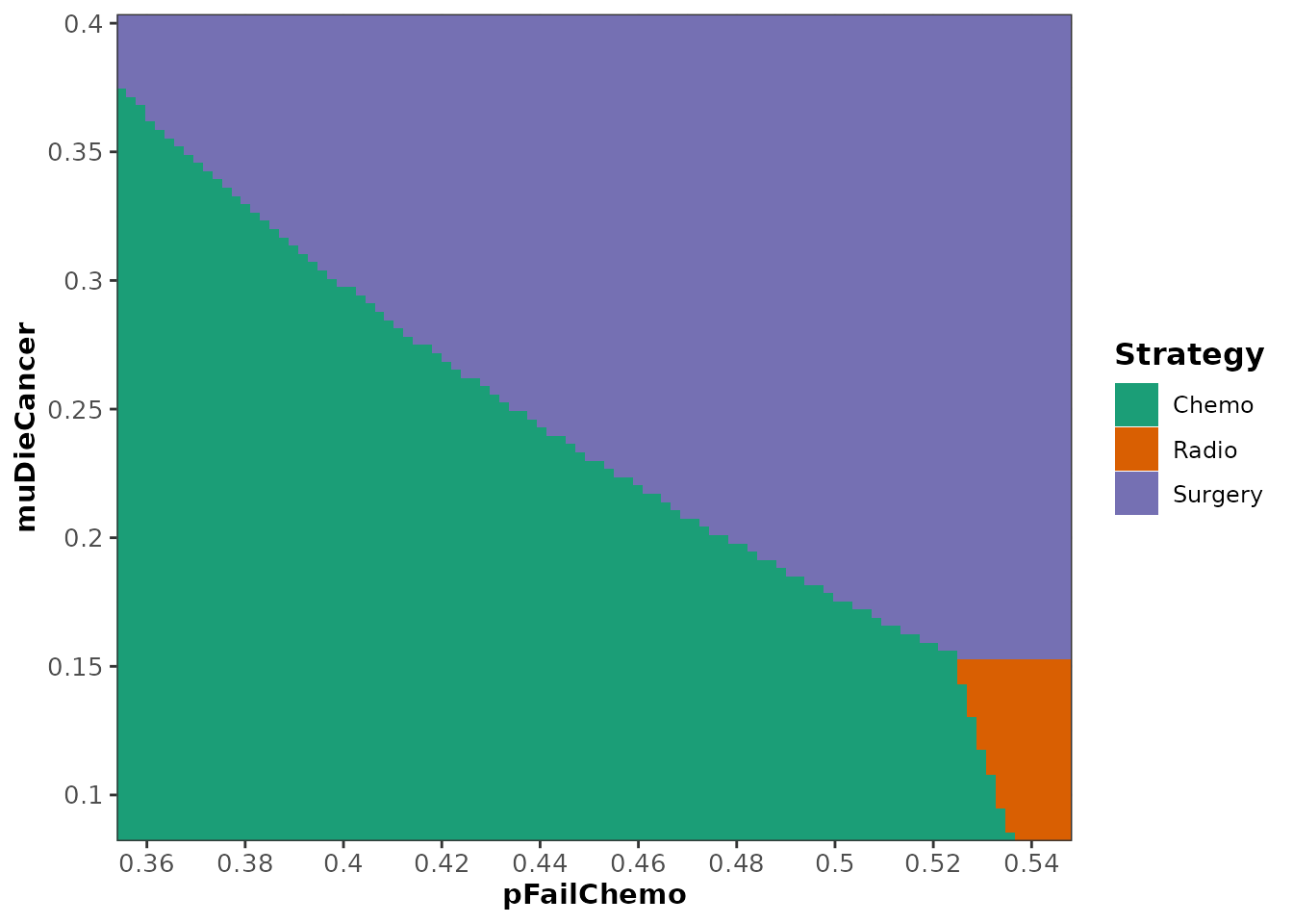
The default plot of a twsa object (see
?plot.twsa) shows the range of the two parameters of
interest on the axes, with each region color coded according to which
strategy maximizes the expected outcome of interest.
plot(twoway_sa_cancer)