This function takes in strategies and their associated cost and effect, assigns them one of three statuses (non-dominated, extended dominated, or dominated), and calculates the incremental cost-effectiveness ratios for the non-dominated strategies
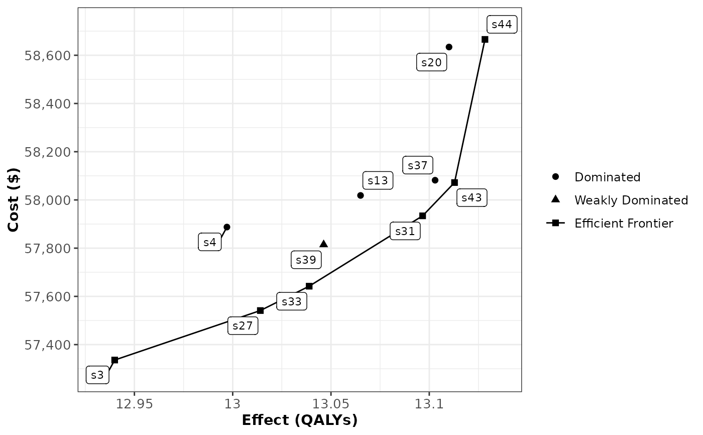
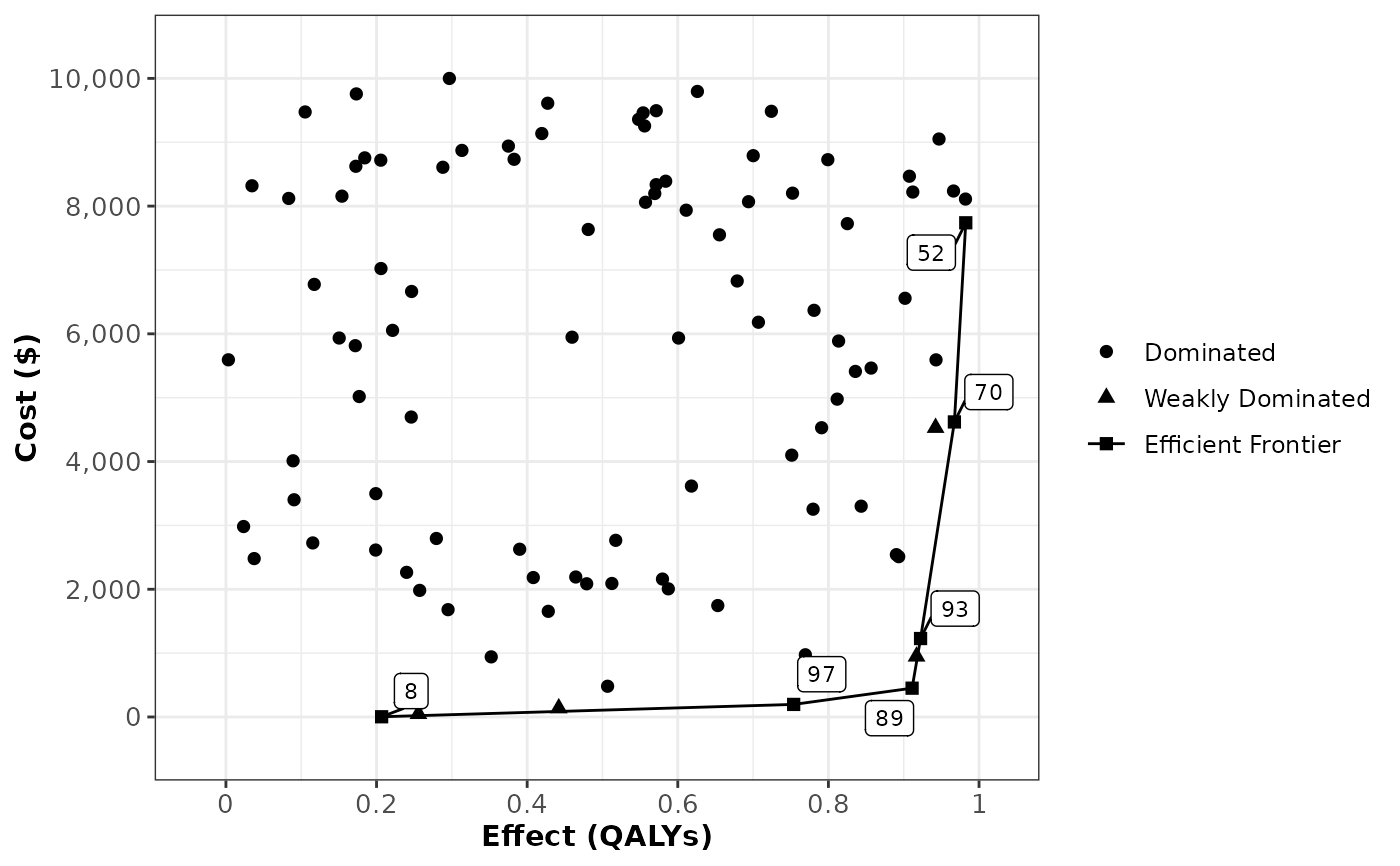
The cost-effectiveness frontier can be visualized with plot, which calls plot.icers.
An efficient way to get from a probabilistic sensitivity analysis to an ICER table
is by using summary on the PSA object and then using its columns as
inputs to calculate_icers.
Value
A data frame and icers object of strategies and their associated
status, incremental cost, incremental effect, and ICER.
Examples
## Base Case
# if you have a base case analysis, can use calculate_icers on that
data(hund_strat)
hund_icers <- calculate_icers(hund_strat$Cost,
hund_strat$QALYs,
hund_strat$Strategy)
plot(hund_icers)
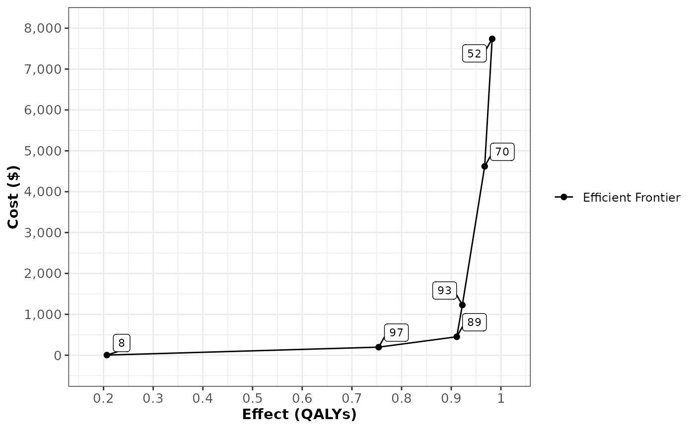
 # we have so many strategies that we may just want to plot the frontier
plot(hund_icers, plot_frontier_only = TRUE)
 # see ?plot.icers for more options
## Using a PSA object
data(psa_cdiff)
# summary() gives mean cost and effect for each strategy
sum_cdiff <- summary(psa_cdiff)
# calculate icers
icers <- calculate_icers(sum_cdiff$meanCost,
sum_cdiff$meanEffect,
sum_cdiff$Strategy)
icers
#> Strategy Costs ($) QALYs Incremental Costs ($) Incremental QALYs
#> 1 s3 57,336 12.94 - -
#> 2 s27 57,541 13.01 205 0.074
#> 3 s33 57,642 13.04 101 0.025
#> 4 s31 57,934 13.10 292 0.058
#> 5 s43 58,072 13.11 138 0.016
#> 6 s44 58,666 13.13 594 0.015
#> 7 s39 57,815 13.05 - -
#> 8 s4 57,887 13.00 - -
#> 9 s13 58,019 13.07 - -
#> 10 s37 58,082 13.10 - -
#> 11 s20 58,634 13.11 - -
#> ICER ($/QALY) Status
#> 1 - ND
#> 2 2,770 ND
#> 3 4,065 ND
#> 4 5,056 ND
#> 5 8,504 ND
#> 6 38,363 ND
#> 7 - ED
#> 8 - D
#> 9 - D
#> 10 - D
#> 11 - D
# visualize
plot(icers)
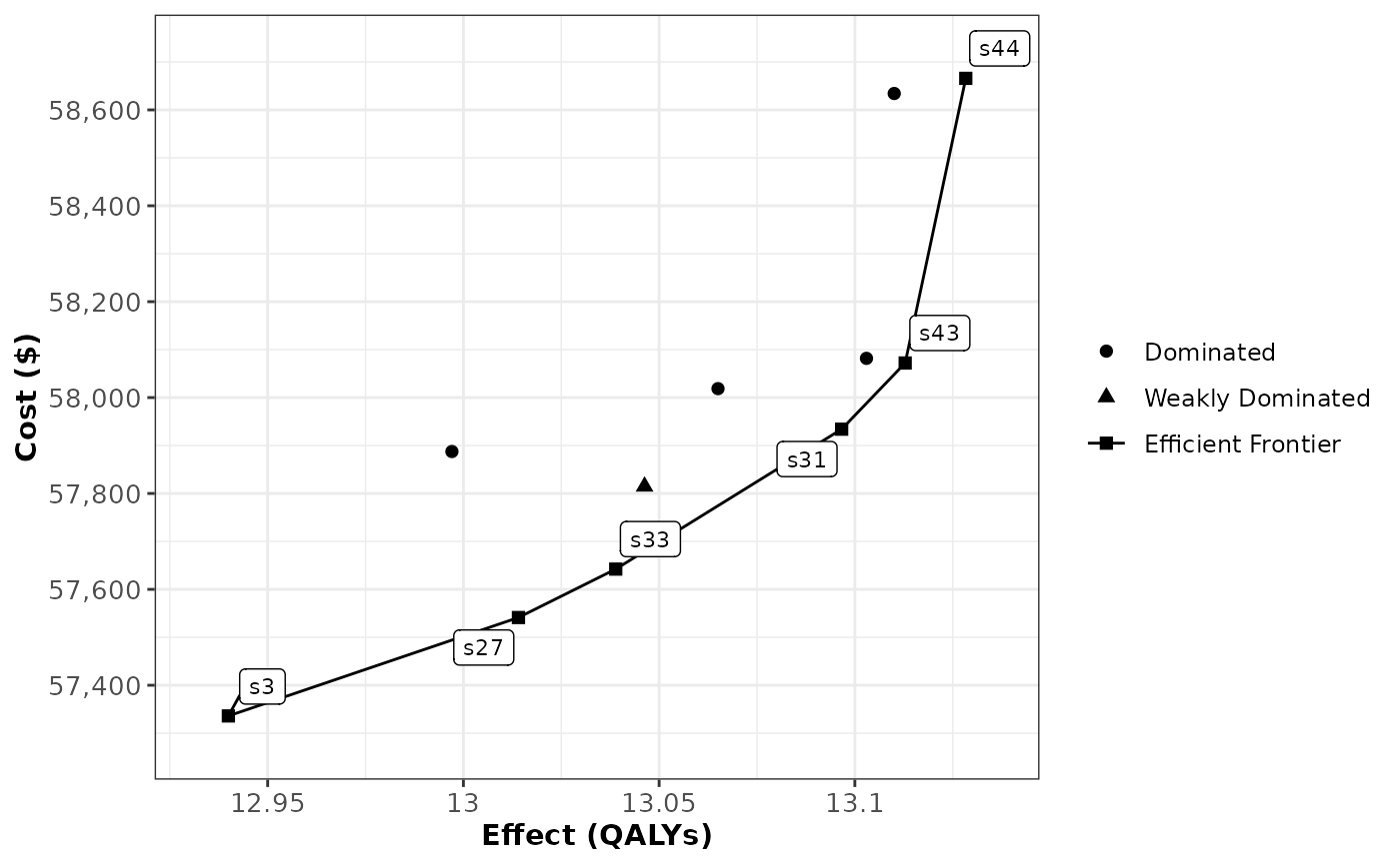 # by default, only the frontier is labeled
# if using a small number of strategies, you can label all the points
# note that longer strategy names will get truncated
plot(icers, label = "all")