Six-strategy PSA sample with a multiply-switching frontier
Source:R/data_example_psa_elc.R
df_example_psa_elc.RdSimulated costs and QALYs for six mutually exclusive strategies, kept in the
package because the resulting cost-effectiveness frontier changes optimal
strategy three times over a plausible willingness-to-pay range. Most bundled
examples switch at most once, which hides defects in the functions that
summarize intervals of optimal choice - the reason
summary.ceac could return duplicated and NA-range rows
unnoticed until 2026 (see the package NEWS for issue #173).
Format
A data frame with 10,000 rows and 12 columns, one row per PSA sample.
Costs occupy columns 1 to 6 and effects columns 7 to 12, so the two halves can
be handed straight to make_psa_obj.
- Cost_1
simulated cost of strategy 1
- Cost_2
simulated cost of strategy 2
- Cost_3
simulated cost of strategy 3
- Cost_4
simulated cost of strategy 4
- Cost_5
simulated cost of strategy 5
- Cost_6
simulated cost of strategy 6
- QALY_1
simulated QALYs of strategy 1
- QALY_2
simulated QALYs of strategy 2
- QALY_3
simulated QALYs of strategy 3
- QALY_4
simulated QALYs of strategy 4
- QALY_5
simulated QALYs of strategy 5
- QALY_6
simulated QALYs of strategy 6
Source
De-identified from a probabilistic analysis of a published decision model. Strategy labels are generic and the underlying parameter draws have been removed, so the sample supports cost-effectiveness analysis but not metamodeling or EVPPI. Costs are rounded to the cent and effects to six decimal places, which leaves every frontier switch point unchanged.
The export it was built from interleaved the two outcomes, with costs in its
even-numbered columns 2 to 12 and QALYs in its odd-numbered columns 3 to 13;
its remaining 34 columns held the parameter draws and were dropped. Here the
two outcomes are separated rather than interleaved, and the source column
names, which were inconsistent, were regularized to Cost_1 to
Cost_6 and QALY_1 to QALY_6.
Details
It is also the sample used to develop the expected loss curve, which is what
the elc suffix refers to.
See also
cancer_psa_data for a three-strategy sample that
also includes the parameter draws.
Examples
data(df_example_psa_elc)

l_psa <- make_psa_obj(cost = df_example_psa_elc[, 1:6],
                      effectiveness = df_example_psa_elc[, 7:12])

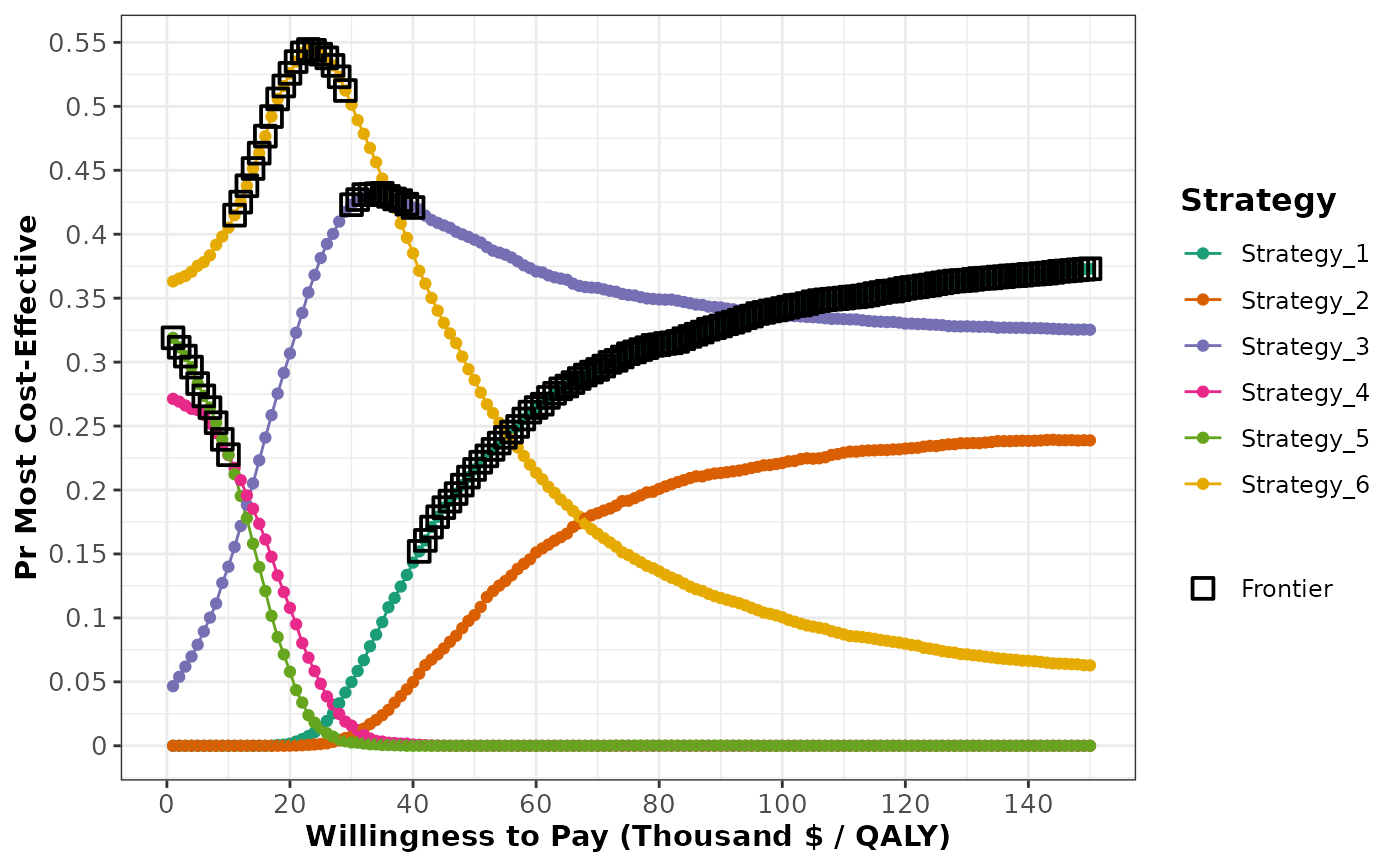
# the frontier switches three times, so the summary has four intervals
df_ceac <- ceac(wtp = seq(1000, 150000, 1000), psa = l_psa)
summary(df_ceac)
#>   range_min range_max optimal_strategy
#> 1      1000     11000       Strategy_5
#> 2     11000     30000       Strategy_6
#> 3     30000     41000       Strategy_3
#> 4     41000    150000       Strategy_1

# the strategy most likely to be cost effective is not necessarily the one
# on the frontier - the plot shows both
plot(df_ceac, frontier = TRUE)